Robot Physics Simulation Basics
Let us learn how to tune some important simulation parameters. Most of the content is based on the following excellent lecture by Dr Russ Tedrake:
The basic dynamics equation for physics is:
\[M(\mathbf{q}) \ddot{\mathbf{q}} + C(\mathbf{q}, \dot{\mathbf{q}}) \dot{\mathbf{q}} = \mathbf{u} + \tau_g \left( \mathbf{q} \right) + \sum_{c \in \mathcal{C}} J_c^T \left( \mathbf{q} \right) F_c\]where
- $\mathbf{q}$ is the vector of all DoF positions
- $M$ is the mass matrix
- $C$ is the coriolis term
- $\mathbf{u}$ is the control input (generalized force) at each DoF
- $\tau_g$ is the gravity force
- $\mathcal{C}$ is the set of contacts $c$ whose Jacobians are $J_c$, and
- $F_c$ is the contact wrench in the task space.
Usually, all DoFs are compensated for gravity and coriolis forces, and driven to some target using PD control. In addition, we have some feedforward acceleration $\ddot{\mathbf{q}}_d$. Hence the conrol input is of the form
\[\mathbf{u} = M(\mathbf{q}) \ddot{\mathbf{q}}_d + C(\mathbf{q}, \dot{\mathbf{q}}) \dot{\mathbf{q}} - \tau_g \left( \mathbf{q} \right) + K_P \left( \mathbf{q}_d - \mathbf{q} \right) + K_D \left( \dot{\mathbf{q}}_d - \dot{\mathbf{q}}\right)\]Assuming for now that we do not have any external contacts (all $F_c$ are 0), and substituting $\mathbf{u}$ we get
\[M(\mathbf{q}) \left( \ddot{\mathbf{q}}_d - \ddot{\mathbf{q}} \right) = -K_P \left( \mathbf{q}_d - \mathbf{q} \right) - K_D \left( \dot{\mathbf{q}}_d - \dot{\mathbf{q}}\right)\]This formulation of the control input linearizes the system. This might explain why PD control on robot DoFs is so popular, and also why MuJoCo (a popular physics simulator) has a soft (PD) constraint model. Setting $\mathbf{e} = \mathbf{q}_d - \mathbf{q}$ we get
\[M(\mathbf{q}) \ddot{\mathbf{e}} = -K_P \mathbf{e} - K_D \dot{\mathbf{e}}\]Setting $\mathbf{x} = \begin{bmatrix} \mathbf{e} \ \dot{\mathbf{e}} \end{bmatrix}^T$ we can write the above in matrix form as
\[\dot{\mathbf{x}} = \begin{bmatrix} \dot{\mathbf{e}} \\ \ddot{\mathbf{e}} \end{bmatrix} = \begin{bmatrix} 0 & 1 \\ -M^{-1} K_P & -M^{-1} K_D \end{bmatrix} \begin{bmatrix} \mathbf{e} \\ \dot{\mathbf{e}} \end{bmatrix} = A \mathbf{x}\]Switching to the scalar version for simplicity, we can analyze the stability of the above linear system by looking at the real parts of the eigenvalues of $A$, which are the the roots of $det \left( \lambda I - A \right) = 0$. The eigenvalues are
\[\lambda = \frac{-K_D + \sqrt{K_D^2 - 4 M K_P}}{2 M}\]If $K_P$, $K_D$, and $M$ are all positive (which are reasonable assumptions), the system is stable because the real parts of the eigenvalues of $A$ are negative.
Discrete Time
All this is nice, but simulations have to discretize time. They can use $\dot{\mathbf{x}}$ from the continuous time calculation above, but at the end of the day they have to report the state $\mathbf{x}$ at discrete time intervals. The equation can be solved theoretically in a closed form but this involves an integration which is again inevitably discretized while computing. In practice, simulators use much more simple approximations. We discuss Euler integration below, but others like backward Euler and Runge-Kutta also have similar properties (I think).
In Euler’s integration, we make the following simplification:
\[\mathbf{x} [n+1] = \mathbf{x} [n] + h \dot{\mathbf{x}} [n] = \mathbf{x} [n] + h A [n] \mathbf{x} [n] = \left( I + h A [n] \right)\mathbf{x} [n]\]where $h$ is the simulation timestep. Eigenvalues $\lambda$ are the roots of
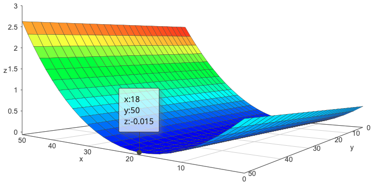
\[\begin{align*} det \left( \lambda I - \left( I + h \begin{bmatrix} 0 & 1 \\ -\frac{K_P}{M} & -\frac{K_D}{M} \end{bmatrix} \right) \right) &= 0 \\ \implies det \left( \begin{bmatrix} \lambda & 0 \\ 0 & \lambda \end{bmatrix} - \begin{bmatrix} 1 & h \\ -\frac{h K_P}{M} & 1 - \frac{h K_D}{M} \end{bmatrix} \right) &= 0 \\ \implies det \left( \begin{bmatrix} \lambda - 1 & -h \\ \frac{h K_P}{M} & \lambda - 1 + \frac{h K_D}{M} \end{bmatrix} \right) &= 0 \\ \implies \left( \lambda - 1 \right) \left( \lambda - 1 + \frac{h K_D}{M} \right) + \frac{h^2 K_P}{M} &= 0 \\ \implies \lambda^2 - \lambda \left( 2 - \frac{h K_D}{M} \right) + \left( 1 - \frac{h K_D}{M} + \frac{h^2 K_P}{M} \right) &= 0 \end{align*}\]The real part of $\lambda$ is $Re(\lambda) = \frac{2 - \frac{h K_D}{M}}{4 \left( 1 - \frac{h K_D}{M} + \frac{h^2 K_P}{M} \right)}$. The condition for stability of a discrete time system is $\vert Re(\lambda) \vert < 1$. We can see from the below graph of $Re(\lambda)$ (Z axis surface) for $h = 0.1$ that this condition is not always satisfied. The surface plot has $\frac{K_P}{M}$ on the Y axis and $\frac{K_D}{M}$ on the X axis.
Conclusions
In discrete time (i.e. almost all physics simulators) the choice of time constant and PD control gains needs to be carefully thought out. Dr Tedrake recommends the following steps to fix unexpected behaviour in a simulator resulting from the kind of instability discussed above:
- Reduce the timestep as much as needed to fix the behaviour
- Identify the source of maximum stiffness ($K_P$) in the system, and reduce it as much as acceptable
- The reduction in stiffness can enable you increase the timestep, making the simulation faster.