Camera-Robot Extrinsic Calibration
These days we are seeing a lot of research in perception for grasping and manipulation of objects with robot arms. For any of these to work, pixels in the camera images need to be connected to 3D points in the robot’s task space.
Camera-Robot Extrinsic calibration solves this problem, and in this blog post I want to talk about the fun matrix algebra behind it. Hand-eye calibration and Eye-on-hand calibration are related terms.
Summary
- Solve $AX=XB$ for hand-eye calibration
- Invert the poses used to construct $A$ for eye-on-hand calibration!
- Additionally invert the poses used to construct $B$ for more interesting information!
Let us consider the following coordinate systems:
-
b: robot base -
e: robot end-effector -
t: calibration target e.g. checkerboard, ArUco marker(s), April tag(s)
Symbols denoting poses follow the
usual
convention:
$^AT_B$ indicates the pose of frame B w.r.t. frame A.
Camera Pose w.r.t. Robot Base a.k.a. Hand-Eye Calibration
Calibration target is rigidly attached to the robot end effector. A static camera observes the end-effector (and calibration target) motion.
- Known: $^cT_t$ (from marker detection in the camera images) and $^bT_e$ (from the robot controller)
- Unknown: $^bT_c$ and $^eT_t$
We are interested in $^bT_c$.
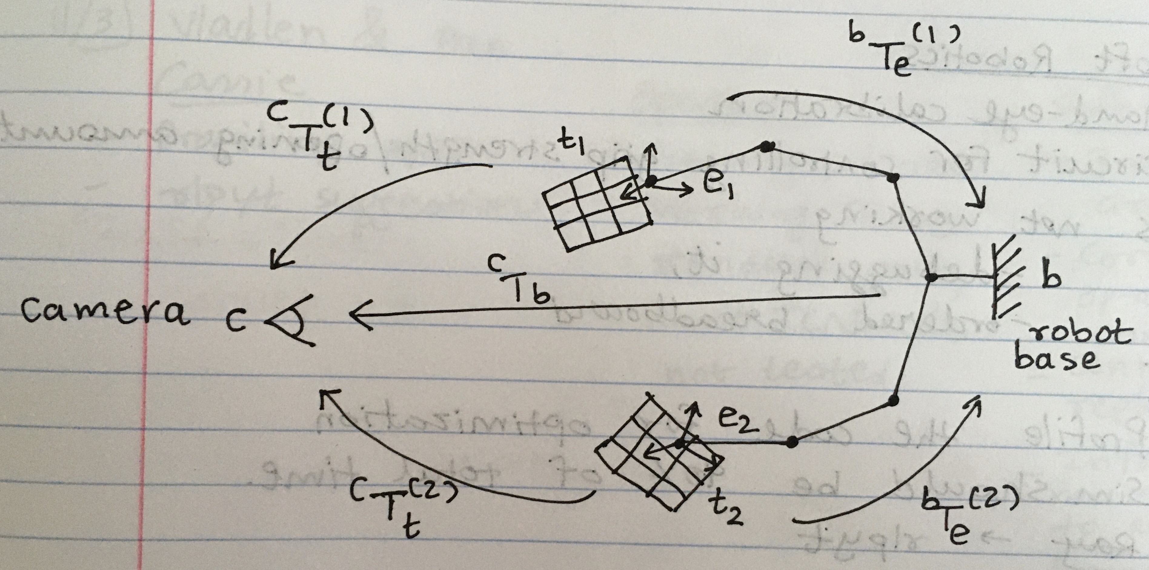
Looking at the figure above, which shows two motions of the robot
((1) and (2)), we can identify the kinematic “cycle”:
Note how cleanly the $A$ terms come from the robot kinematics, $X$ is the unknown, and $B$ terms come from camera marker detection. In practice, more than 2 frames of motion are used to construct $A$ and $B$. The data is then passed to an “$AX=XB$” solver (paper | code).
Camera Pose w.r.t. Robot End-effector a.k.a. Eye-On-Hand Calibration
Calibration target stationary in the world. The camera is rigidly attached to the robot end effector. The camera observes the calibration target from various perspectives through robot arm motion.
- Known: $^cT_t$ (from marker detection in the camera images) and $^bT_e$ (from the robot controller)
- Unknown: $^eT_c$ and $^bT_t$
We are interested in $^eT_c$.
Similar to above, we identify a kinematic “cycle”:
\[\begin{align*} ^bT_e^{(1)}~^eT_c~^cT_t^{(1)} &= ~^bT_e^{(2)}~^eT_c~^cT_t^{(2)}\\ ^eT_b^{(2)}~^bT_e^{(1)}~^eT_c &= ~^bT_c~^cT_t^{(2)}~^tT_c^{(1)} && \text{(Moving $~^cT_t^{(1)}$ to the right, $~^bT_e^{(2)}$ to the left)}\\ \underbrace{^eT_b^{(2)}{~^eT_b^{(1)}}^{-1}}_A \underbrace{~^eT_c}_X &= \underbrace{~^eT_c}_X \underbrace{~^cT_t^{(2)}{~^cT_t^{(1)}}^{-1}}_B && \text{(Inverting $~^bT_e^{(1)}$ and $~^tT_c^{(1)}$)} \end{align*}\]Note how the equation is almost the same as the hand-eye calibration equation above, you just need to invert the robot kinematics data!
Bonus
Let us try to solve for the pose of the calibration target w.r.t robot end-effector, $^eT_t$, in the hand-eye calibration scenario:
\[\begin{align*} ^bT_e^{(1)}~^eT_t~^tT_c^{(1)} &= ~^bT_e^{(2)}~^eT_t~^tT_c^{(2)}\\ ^eT_b^{(2)}~^bT_e^{(1)}~^eT_t &= ~^eT_t~^tT_c^{(2)}~^cT_t^{(1)} && \text{(Moving $~^tT_c^{(1)}$ to the right, $~^bT_e^{(2)}$ to the left)}\\ \underbrace{^eT_b^{(2)}{~^eT_b^{(1)}}^{-1}}_A \underbrace{~^eT_t}_X &= \underbrace{~^eT_t}_X \underbrace{~^tT_c^{(2)}{~^tT_c^{(1)}}^{-1}}_B && \text{(Inverting $~^bT_e^{(1)}$ and $~^cT_t^{(1)}$)} \end{align*}\]So if you invert both robot kinematics and marker detection data in the hand-eye calibration equations, you get the pose of the calibration target w.r.t. robot end effector!
The same reasoning applies to the pose of the calibration target w.r.t. robot base for the eye-on-hand scenario.
Further Steps
The paper I linked above and the code linked below solve the “$AX=XB$” problem in the least-squares sense. You might want to use that solution as initialization for a nonlinear optimization problem, like this paper does. You can use GTSAM or the Ceres solver for that. Why would this improve the solution?
Instead of casting this problem as $AX=XB$, you could cast it as $AX=ZB$, where the $A$ and $B$ matrices are made from poses and not motions. This formulation has some advantages which help in optimization. See this Twitter thread for justifications, and this paper for details.
Code
In spite of being a required basic ingredient for robot grasping research, I was surprised to find that none of the available code worked out of the box. I looked at the following:
There are probably many other repositories but I settled on MoveIt! Calibration because it integrates marker tracking, solver, and robot motion control all in one place. It can record the joint states of your robot that were used for calibration, and then play them back to re-calibrate later if you move your camera. This is a very useful under-appreaciated feature.
Anyway, in this blog I wanted to explain the maths behind the “$AX=XB$” used under the hood of all these repositories, so that you can modify the code yourself if you need to. Also, it is fun to see how you can get completely different output quantities by inverting various input quantities!