6.832 Underactuated Robotics - Lecture 1
Video Lecture | Class Notes
Problem Set
1.1.1
Underactuated, because a purely `sideways’ acceleration in the direction opposing gravity is not possible for any control input. So the map $\ddot q = f(q, \dot q, u, t)$ is not surjective.
1.1.2
If we assume unit mass, length and inertia matrix,
\[\begin{bmatrix} \ddot x \\ \ddot z + g \\ \ddot \theta \end{bmatrix} = \begin{bmatrix} -\sin \theta & -\sin \theta \\ \cos \theta & \cos \theta \\ 1 & -1 \end{bmatrix} \begin{bmatrix}F_1 \\ F_2\end{bmatrix}\]i.e. system is control affine.
Let us take the example of a purely sideways acceleration i.e. \(\begin{align*} & \ddot \theta = 0, \ddot x = a \cos \theta, \ddot z = a \sin \theta\\ &\implies F_1 = F_2 = k (say)\\ &\implies a \cos \theta = -2k \sin \theta, a \sin \theta + g = 2k \cos \theta\\ &\implies a = -g \sin \theta \end{align*}\)
For $\theta = 0.5$, $\sin \theta \approx 0.5$. Hence $a$ cannot be positive. Concretely, $\ddot q = (5 \cos \theta, 5 \sin \theta, 0)$ is not possible instantaneously at $\theta = 0.5$.
1.2.1
In this case,
\[\begin{align*} f_r &= K_1\\ f_f &= K_2 - C_f \phi\\ I\ddot \theta &= -b f_r + a f_f \cos \phi\\ &= -bK_1 + a K_2 \cos \phi - a C_f \phi \cos \phi\\ m \ddot x &= K_3 - f_f \sin(\theta + \phi) + u_r \cos \theta\\ &= K_3 - K_2 \sin(\theta + \phi) + C_f \phi \sin(\theta + \phi) + u_r \cos \theta\\ m \ddot y &= K_4 + f_f \cos(\theta + \phi) + u_r \sin \theta\\ &= K_4 + K_2 \cos(\theta + \phi) - C_f \phi \cos(\theta + \phi) + u_r \sin \theta\\ \implies \begin{bmatrix}I\ddot \theta \\ m \ddot x\\ m \ddot y\end{bmatrix} &= \begin{bmatrix} -bK_1 + a K_2 \cos \phi\\ K_3 - K_2 \sin(\theta + \phi)\\ K_4 + K_2 \cos(\theta + \phi) \end{bmatrix} + \begin{bmatrix} -a C_f \cos \phi & 0\\ C_f \sin(\theta + \phi) & \cos \theta\\ -C_f \cos(\theta + \phi) & \sin \theta \end{bmatrix} \begin{bmatrix}\phi \\ u_r\end{bmatrix} \end{align*}\]which means the system is control-affine. The $B$ matrix has shape 2 $\times$ 3, while dim($q$) = 3, which means the system is underactuated.
1.2.2
Intuitively, the system is still underactuated because of holonomic constraints. An acceleration of the type $(\ddot x, \ddot y, \ddot \theta) = (0, k, 0)$ is not possible instantaneously.
1.2.3
When $\phi_0 = 0$
\[f_2(q, \dot q, t) = \begin{bmatrix} -a C_f & 0 & 0\\ -C_f arctan\left( \frac{\dot y + \dot \theta a}{\dot x} \right) & 1 & 1\\ -C_f & 0 & 0 \end{bmatrix}\]which has rank 2 because rows 1 and 2 are not linearly independent.
1.2.4
row 1 = $a \times$ row 3, so they will never be linearly independent. Hence there are no values of $\phi_0$ for which the linearized system is fully actuated.
1.3.1
- No, we need the position and velocity of center of mass (or any other well defined point on the robot body) in the state as well.
- False, because no control input can produce a (large) vertical acceleration in the COM.
- False, because pure in-place rotation acceleration of the COM or acceleration the COM along the straight line are not possible.
2.1
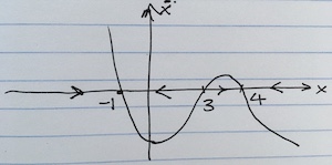
$(-1, 0), (3, 0)$ and $(4, 0)$ are equilibrium points.
2.2
- $x = 1$ - stable - basin of attraction $(-\infty, 3)$
- $x = 3$ - unstable
- $x = 4$ - stable - basin of attraction $(3, \infty)$
3.1
Following the example from 2, let $\dot x = f(x) = -x^3 + 6 x^2 - 5 x - 12$, $x^* = -1$. Note that $f(x^*) = 0, \pdv{f(x^*)}{x} = -20 < 0$
Now, if $x[k-1] = -2$,
\[\begin{align*} x[k] &= -2 + h f(-2)\\ \implies x[k] &= -2 + 30 h\\ \end{align*}\]so $x[k] = 3.5$ for $h = 0.183$. Now $f(3.5) = 1.125 > 0$, so $x=-1$ is not stable. Intuitively, an arbitrarily large time step $h$ allows one to jump an equilibrium point.
3.2
$x[k] = x^* = x[k-1] + h f(x[k-1])$. Linearizing $f(x)$, $f(x[k-1]) = f(x^*) + \pdv{f(x*)}{x}(x[k-1]-x^*) = \pdv{f(x*)}{x}(x[k-1]-x^*)$.
Hence, $x[k] = x[k-1] + h (x[k-1]-x[k])\pdv{f(x[k])}{x}$. If we want $x[k]$ to not ‘skip’ = $x^*$, then $h < \frac{1}{\vert \pdv{f(x[k])}{x} \vert} = \frac{1}{G}$.
4.2.1
Manipulator equations: $M(q, \dot q)\ddot q + C(q, \dot q)\dot q = \tau_g + Bu$. With the following feedback linearization,
\[u = B^{-1}\left[ M\ddot q - \tau_g + C \dot q_d \right]\]we have $\dot q = \dot q_d$. If $q_0 = q_d(0)$, then $q(t) = q_d(t) \forall t \geq 0$.
4.2.2
Manipulator equations: $M(q, \dot q)\ddot q + C(q, \dot q)\dot q = \tau_g + Bu$. With the following feedback linearization,
\[u = B^{-1}\left[ M\ddot q_d - \tau_g + C \dot q \right]\]we have $\ddot q = \ddot q_d$. If $\dot q_0 = \dot q_d(0)$, then $\dot q(t) = \dot q_d(t) \forall t \geq 0$.
4.2.3
Yes, see 4.2.2 above.
4.3
We are given the dynamics,
\[\ddot \theta = -\frac{g}{l}\sin\theta - \frac{C}{l}\omega^2\sin(\omega t)\cos\theta + \frac{u}{m l^2}\]Picking the feedback linearization
\[u = m l^2 \left( -\dot\theta + 1 + \frac{g}{l}\sin\theta + \frac{C}{l}\omega^2\sin(\omega t)\cos\theta \right)\]we get $\ddot\theta = -\dot\theta + 1$.
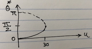
5.1.1
System becomes unstable when $u \geq 30$.
5.1.2
The equations of motion are $m l^2 \ddot\theta + b \dot\theta + m g l \sin\theta = u$.
5.1.2
When $u > 30$, $u$ dominates $m g l \sin\theta$, so $m l^2 \ddot\theta \approx -b \dot\theta + u$.
Hence we have a dynamical system $3 \dot x = -2x + 30$, or $\dot x = -\frac{2}{3}x + 10$ which is a stable linear system that converges to
\[\begin{align*} x(t) &= e^{-\frac{2}{3}t}x_0 + \int_{0}^{t} e^{-\frac{2}{3}(t-\tau)} 10 d\tau\\ &= e^{-\frac{2}{3}t}x_0 + 10 e^{-\frac{2}{3}t} \int_{0}^{t} e^{\frac{2}{3}\tau} d\tau\\ &= e^{-\frac{2}{3}t}x_0 + 15 e^{-\frac{2}{3}t} \left( e^{\frac{2}{3}t} - 1 \right)\\ &= 15 + e^{-\frac{2}{3}t}x_0 - 15 e^{-\frac{2}{3}t} \end{align*}\]At $t = \infty$, $x(t) = 15$.
5.2
Tracking plots
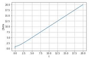
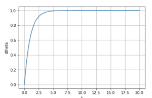
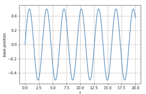
Tracking requires some time to catch up. We can improve the performance by enforcing a PID-type system $\ddot\theta = K_P(\dot\theta-1) + K_I\int (\dot\theta(\tau)-1) d\tau + K_D \ddot\theta$ and tuning the gains $K_P$, $K_I$ and $K_D$.
Equation of motion for a simple pendulum
 Figure from https://underactuated.mit.edu
Position $p = l\begin{bmatrix}\sin \theta \\ \cos \theta\end{bmatrix}$.
Velocity $\dot p = l \dot \theta \begin{bmatrix}\cos \theta \\ -\sin \theta\end{bmatrix}$
Kinetic energy
\[\begin{align*} T &= \frac{1}{2} m \dot p^T \dot p \\ &= \frac{1}{2} m l^2 \dot \theta^2 \end{align*}\]Potential energy $U = -mgl \cos\theta$
Lagrangian “crank”:
\[\begin{align*} \dv{}{t} \pdv{L}{\dot \theta} - \pdv{L}{\theta} &= \tau\\ \implies \dv{}{t} m l^2 \dot\theta - m g l\sin\theta &= \tau\\ \implies m l^2 \ddot\theta - m g l \sin\theta &= \tau \end{align*}\]Equations of motion for a double pendulum (Manipulator Equations)
 figure from http://underactuated.mit.edu/
State $q = \begin{bmatrix}\theta_1 \\ \theta_2\end{bmatrix}$.
Positions of masses $m_1$ and $m_2$ are:
\[p_1 = l_1\begin{bmatrix}s_1 \\\ -c_1 \end{bmatrix}\] \[p_2 = p_1 + l_2\begin{bmatrix}s_{1+2} \\\ -c_{1+2} \end{bmatrix}\]Velocities are:
\[\dot p_1 = l_1 \dot\theta_1 \begin{bmatrix}c_1 \\\ s_1 \end{bmatrix}\] \[\dot p_2 = \dot p_1 + l_2 \left(\dot\theta_1 + \dot\theta_2\right) \begin{bmatrix}c_{1+2} \\\ s_{1+2} \end{bmatrix}\]Total kinetic energy
\[\begin{align*} T &= \frac{1}{2}m_1 \dot p_1^T \dot p_1 + \frac{1}{2}m_2 \dot p_2^T \dot p_2\\ &= \frac{1}{2}m_1 \dot p_1^T \dot p_1 + \frac{1}{2}m_2 \left( \dot p_1^T \dot p_1 + 2 l_2 \left(\dot\theta_1 + \dot\theta_2\right) \dot p_1^T \begin{bmatrix}c_{1+2} \\\ s_{1+2} \end{bmatrix} + l_2^2 \left(\dot\theta_1 + \dot\theta_2\right)^2 \right)\\ &= \frac{1}{2} (m_1 + m_2) l_1^2 \dot \theta_1^2 + m_2 l_1 l_2 \dot\theta_1 \left(\dot\theta_1 + \dot\theta_2\right) (c_1 c_{1+2} + s_1 s_{1+2}) + \frac{1}{2} m_2 l_2^2 \left(\dot\theta_1 + \dot\theta_2\right)^2 \\ &= \frac{1}{2} (m_1 + m_2) l_1^2 \dot \theta_1^2 + c_2 m_2 l_1 l_2 \dot\theta_1 \left(\dot\theta_1 + \dot\theta_2\right)+ \frac{1}{2} m_2 l_2^2 \left(\dot\theta_1 + \dot\theta_2\right)^2 \end{align*}\]Total potential energy
\[\begin{align*} U &= m_1 g y_1 + m_2 g y_2\\ &=-g\left(m_1 l_1 c_1 + m_2(l_1 c_1 + l_2 c_{1+2}) \right) \end{align*}\]The Lagrangian is $L = T - U$
Lagrangian equation of the first kind for $\theta_1$:
\[\dv{}{t} \pdv{L}{\dot \theta_1} - \pdv{L}{\theta_1} = \tau_1\]Now
\[\begin{align*} \pdv{L}{\dot \theta_1} &= \pdv{}{\dot \theta_1} \left[ \frac{1}{2} (m_1 + m_2) l_1^2 \dot \theta_1^2 + c_2 m_2 l_1 l_2 \dot\theta_1 \left(\dot\theta_1 + \dot\theta_2\right)+ \frac{1}{2} m_2 l_2^2 \left(\dot\theta_1 + \dot\theta_2\right)^2 + g\left(m_1 l_1 c_1 + m_2(l_1 c_1 + l_2 c_{1+2}) \right) \right]\\ &= (m_1 + m_2) l_1^2 \dot \theta_1 + c_2 m_2 l_1 l_2 (2\dot\theta_1 + \dot\theta_2) + m_2 l_2^2 \left(\dot\theta_1 + \dot\theta_2\right) \end{align*}\]Hence
\[\begin{align*} \dv{}{t} \pdv{L}{\dot \theta_1} &= \dv{}{t} \left[ (m_1 + m_2) l_1^2 \dot \theta_1 + c_2 m_2 l_1 l_2 (2\dot\theta_1 + \dot\theta_2) + m_2 l_2^2 \left(\dot\theta_1 + \dot\theta_2\right) \right] \\ &= (m_1 + m_2) l_1^2 \ddot \theta_1 + m_2 l_2^2 \left(\ddot\theta_1 + \ddot\theta_2\right) + m_2 l_1 l_2 (2\ddot\theta_1 + \ddot\theta_2) c_2 - m_2 l_1 l_2 (2\dot\theta_1 + \dot\theta_2) \dot \theta_2 s_2 \end{align*}\]And
\[\begin{align*} \pdv{L}{\theta_1} &= \pdv{}{\theta_1} \left[ \frac{1}{2} (m_1 + m_2) l_1^2 \dot \theta_1^2 + c_2 m_2 l_1 l_2 \dot\theta_1 \left(\dot\theta_1 + \dot\theta_2\right)+ \frac{1}{2} m_2 l_2^2 \left(\dot\theta_1 + \dot\theta_2\right)^2 + g\left(m_1 l_1 c_1 + m_2(l_1 c_1 + l_2 c_{1+2}) \right) \right]\\ &= -g \left(m_1 l_1 s_1 + m_2 \left(l_1 s_1 + l_2 s_{1+2} \right) \right) \\ &= -(m_1 + m_2) l_1 g s_1 - m_2 g l_2 s_{1+2} \end{align*}\]Hence we get the Lagrangian equation
\[\begin{equation*} \boxed{ (m_1 + m_2) l_1^2 \ddot \theta_1 + m_2 l_2^2 \left(\ddot\theta_1 + \ddot\theta_2\right) + m_2 l_1 l_2 (2\ddot\theta_1 + \ddot\theta_2) c_2 - m_2 l_1 l_2 (2\dot\theta_1 + \dot\theta_2) \dot \theta_2 s_2 + (m_1 + m_2) l_1 g s_1 + m_2 g l_2 s_{1+2} = \tau_1 } \end{equation*}\]Similarly, Lagrangian equation of the first kind for $\theta_2$:
\[\dv{}{t} \pdv{L}{\dot \theta_2} - \pdv{L}{\theta_2} = \tau_2\]Now
\[\begin{align*} \pdv{L}{\dot \theta_2} &= \pdv{}{\dot \theta_2} \left[ \frac{1}{2} (m_1 + m_2) l_1^2 \dot \theta_1^2 + c_2 m_2 l_1 l_2 \dot\theta_1 \left(\dot\theta_1 + \dot\theta_2\right)+ \frac{1}{2} m_2 l_2^2 \left(\dot\theta_1 + \dot\theta_2\right)^2 + g\left(m_1 l_1 c_1 + m_2(l_1 c_1 + l_2 c_{1+2}) \right) \right]\\ &= c_2 m_2 l_1 l_2 \dot\theta_1 + m_2 l_2^2 \left(\dot\theta_1 + \dot\theta_2\right) \end{align*}\]Hence
\[\begin{align*} \dv{}{t} \pdv{L}{\dot \theta_2} &= \dv{}{t} \left[ c_2 m_2 l_1 l_2 \dot\theta_1 + m_2 l_2^2 \left(\dot\theta_1 + \dot\theta_2\right) \right] \\ &= c_2 m_2 l_1 l_2 \ddot\theta_1 - s_2 m_2 l_1 l_2 \dot\theta_1 \dot\theta_2 + m_2 l_2^2 \left(\ddot\theta_1 + \ddot\theta_2\right) \end{align*}\]And
\[\begin{align*} \pdv{L}{\theta_2} &= \pdv{}{\theta_2} \left[ \frac{1}{2} (m_1 + m_2) l_1^2 \dot \theta_1^2 + c_2 m_2 l_1 l_2 \dot\theta_1 \left(\dot\theta_1 + \dot\theta_2\right) + \frac{1}{2} m_2 l_2^2 \left(\dot\theta_1 + \dot\theta_2\right)^2 + g\left(m_1 l_1 c_1 + m_2(l_1 c_1 + l_2 c_{1+2}) \right) \right]\\ &= -s_2 m_2 l_1 l_2 \dot\theta_1 \left(\dot\theta_1 + \dot\theta_2\right) - g m_2 l_2 s_{1+2} \end{align*}\]Hence we get the Lagrangian equation
\[c_2 m_2 l_1 l_2 \ddot\theta_1 - s_2 m_2 l_1 l_2 \dot\theta_1 + \dot\theta_2 m_2 l_2^2 \left(\ddot\theta_1 + \ddot\theta_2\right) + s_2 m_2 l_1 l_2 \dot\theta_1 \left(\dot\theta_1 + \dot\theta_2\right) + g m_2 l_2 s_{1+2} = \tau_2\] \[\begin{equation*} \boxed{\implies m_2 l_2^2 \left(\ddot\theta_1 + \ddot\theta_2\right) + m_2 l_1 l_2 \ddot\theta_1 c_2 + m_2 l_1 l_2 \dot\theta_1^2 + m_2 g l_2 s_{1+2} = \tau_2 } \end{equation*}\]The Lagrangian equations match the notes and follow the canonical form of manipulator equations
\[M(q) \ddot q + C(q, \dot q)\dot q = \tau_g(q) + Bu\]